")
Introduction
When processing THEMIS images using our web interface, we require that users specify a region of interest by creating a project. This requirement makes the processing of the images more efficient because for each project we produce region specific files, rather than requiring the use of global maps for every image processed. These files consist of maps of elevation, and other interesting data, so they are likely to be of interest to researchers on their own, aside from their critical importance in processing the THEMIS images. For this reason we make the files available to view and download.
Users Guide
To create a project all you need do is specify a region on the Martian surface. We recommend specifying a region no larger than 2 or 3 degrees wide. If you want to specify a larger region in order to generate elevation or TES inertial maps of that region then that is also fine, but we don't want users to specify for example a hemisphere wide project and then process entire long themis images within it. We don't currently prevent that sort of activity, but if it occurs often enought that it begins to affect procesing times for other users then we may have to place limits on processing ranges in the future.
The dust opacity range is the region within which we gather measurements to build the Dust Opacity History. By default it will be the same region as your processing range, but you can also specify a different region. For example you might have several projects centred around different individual features on one part of the planet, and you might want all of those projects to use the same dust history for a region that stradles all the features.
Measurement Types
TES Dust Opacity History
The MARSTHERM THEMIS processing uses as its input data the THEMIS radiance images. From this it is necessary to first derive brightness temperature and then to estimate the actual temperature of the surface, before calculating thermal inertia using the procedure outlined in the THEMIS Processing Documentation. The brightness temperature is a function of the surface temperature attenuated by absorption at the spectral wavelength of the image used. We use band 9 of THEMIS IR images, corresponding to a wavelength of 12.57 µm. At this wavelength the amount of dust in the atmosphere affects the derived brightness temperature, and therefore has an effect on the final derived thermal inertia of surfaces. Measurements of opacity at this wavelength are derived from observations by the Thermal Emission Spectrometer (TES) onboard the Mars Global Surveyor (MGS). Although MGS was in operation around Mars from September 1997 until November 2006, the TES spectrometer (but not the bolometer) failed before contact was lost with the spacecraft. The 2001 Mars Odyssey mission, which houses THEMIS, arrived in October 2001, and the first THEMIS images available come from February 2002 (Spacecraft Clock Time 698,600,000 seconds) so only the last few years of TES data are used when processing THEMIS images.
For the region of interest we find all TES dust opacity measurements, and store them in arrays alongside the space craft clock time and the solar longitude at the time the images were taken. We require at least 2000 measurements within the region, and if after going through every TES data file we do not have that many datapoints then we double the size of the region and start over. This is why the dust opacity range associated with your project may not be the same as the region you requested. We recommend that you request the same dust opacity region as your general processing region, but we allow you the option to specify a different region.
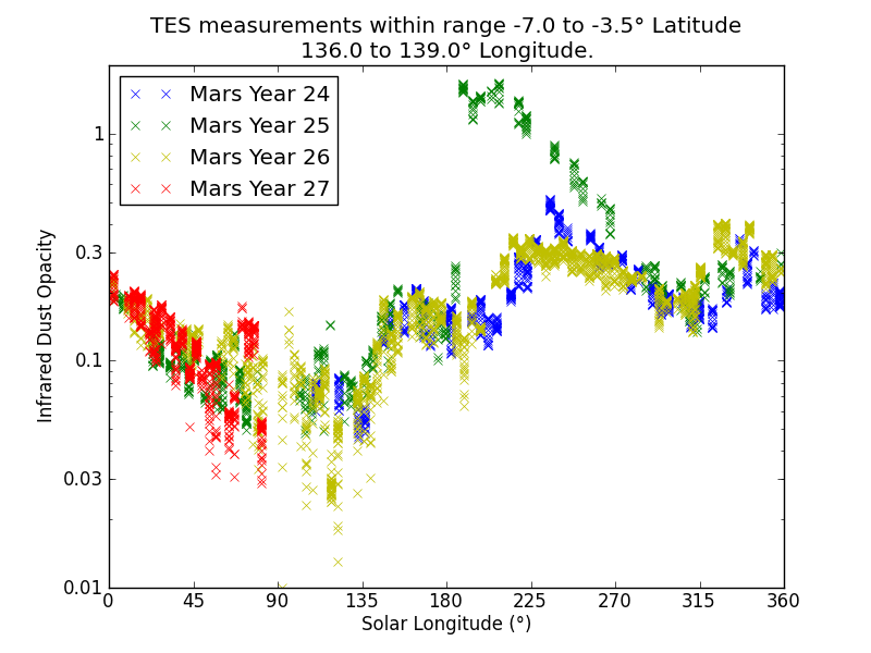
Above plot shows the dust opacity history for a project centred around Gale Crater. The value used by the THEMIS processing algorithm depends on the time when the THEMIS image was taken. If the image was taken before the end of the TES instruments life then a weighted mean of the 5 measurements closest to the appropriate Spacecraft Clock Time is used. If the image was taken after this time then the median value of all measurements falling within 1 degree of Solar Longitude is used. To emphasize:
- for early images actual measurements of opacity at or near to that time are used.
- for later images it is assumed that opacity is seasonaly dependent, and a mediam value for that season is used.
Elevation Map
The amount by which the dust opacity attenuates the infrared radiation reaching the THEMIS camera from the Martian surface also depends on how much atmosphere lies between the two, i.e. it also depends on the elevation of the point. So an elevation map is also required to scale dust opacity. It is assumed that the dust opacity at the 6.1-mbar level is constant across the entire project processing range, so that the only differences in dust opacity per pixel of an image are due to elevation. Elevation maps are also used to calculate the slope of surfaces. We use MOLA elevation maps at 20 pixels per degree. We crop the maps to within 1.5 degrees of the requested range and save that array as an elevation map file, from which elevations for every pixel in any THEMIS image are interpolated linearly.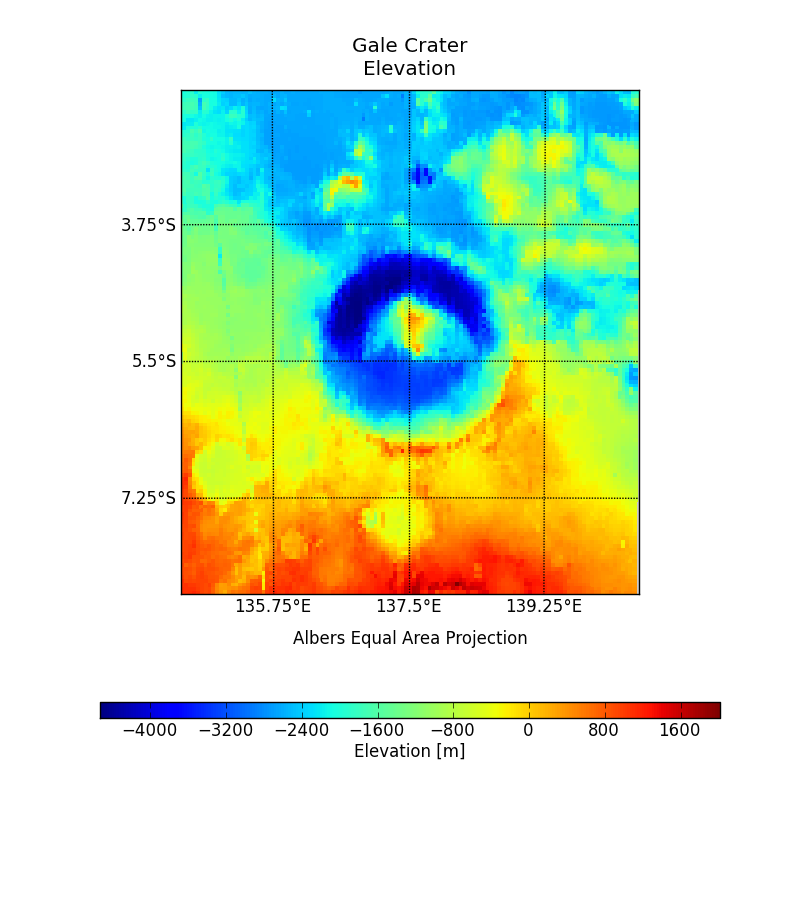
Above plot shows the elevation for the same Gale Crater project. The image is trimmed to the requested range, but as stated the map file will contain an additional 1.5 degree band on each side. This is to ensure that pixels to the edge have enough data to interpolate from.
TES Albedo Maps
The derived thermal inertia of a surface also depends on the surfaces albedo. If a surface has a higher albedo than expected then it will not absorb as much Sun light as expected, so it's surface temperature will not be correctly modelled and therefore neither will it's thermal inertia. Albedo is another value that was measured by the TES instrument but not by THEMIS, it is also time dependent. The dust history map above shows that a number of dust storms came through during the TES instruments life time, and lifted and deposited dust, changing the albedo of different surfaces in different ways. In fact most of these dust storms were planet wide. Large dust storms enveloped the planet twice during the period when both THEMIS and TES were operational, in April 2002 (Spacecraft Clock Time 704,100,000 seconds) and in April 2004 (Spacecraft Clock Time 756,500,000 seconds). The temporal change in albedo is gradual between dust storms, but can be dramatic during a storm so three albedo maps are used for processing of THEMIS images, one for images taken before the first storm, one for between the first and second storms, and one for all images taken after the final dust storm that occured during the TES instruments life time. The albedo used for THEMIS images taken after the failure of the TES instrument may be inaccurate. The maps of TES measured albedo are generated automatically and may, due to the vagueries of the Mars Global Surveyer's orbital path, have left large regions of your processing region un-sampled, for one map or another, this may result in large artifacts when the maps are interpolated to pixel locations in your THEMIS images. You should take a careful look at your albedo maps and decide if they are adequate throughout the region you specified. If they are not then you may wish to download the maps (or find maps of your own), process them some how (by, for example, stacking one on top of another), and e-mail us the corrected maps in the same form as those that you downloaded.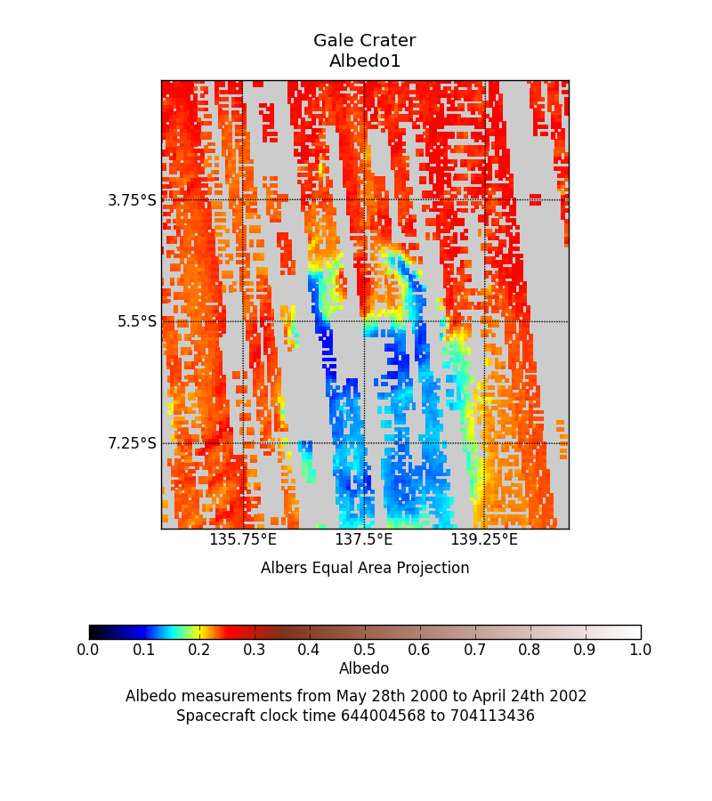
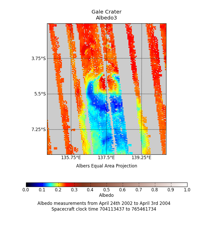
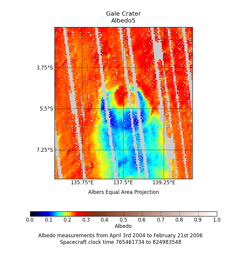
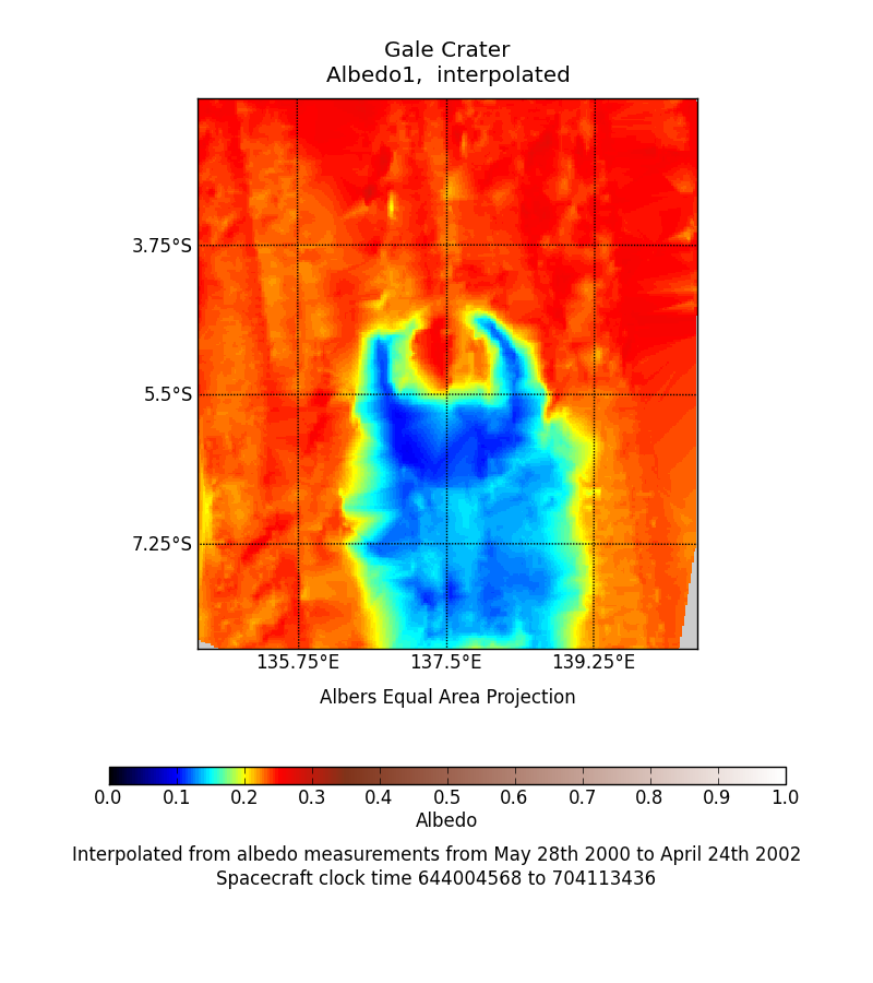
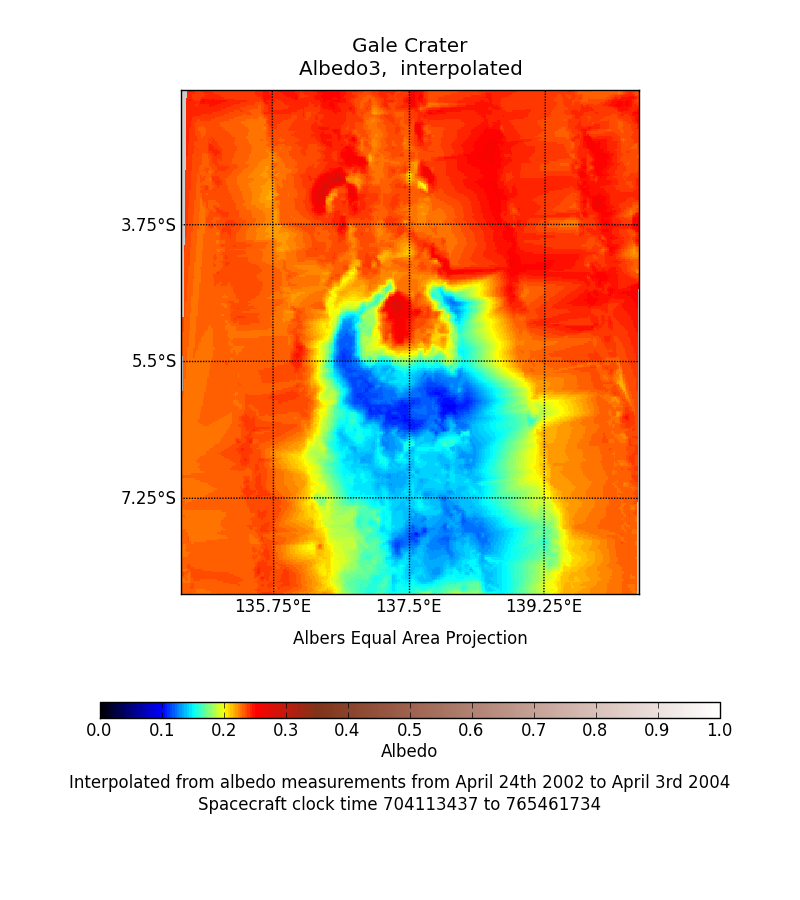
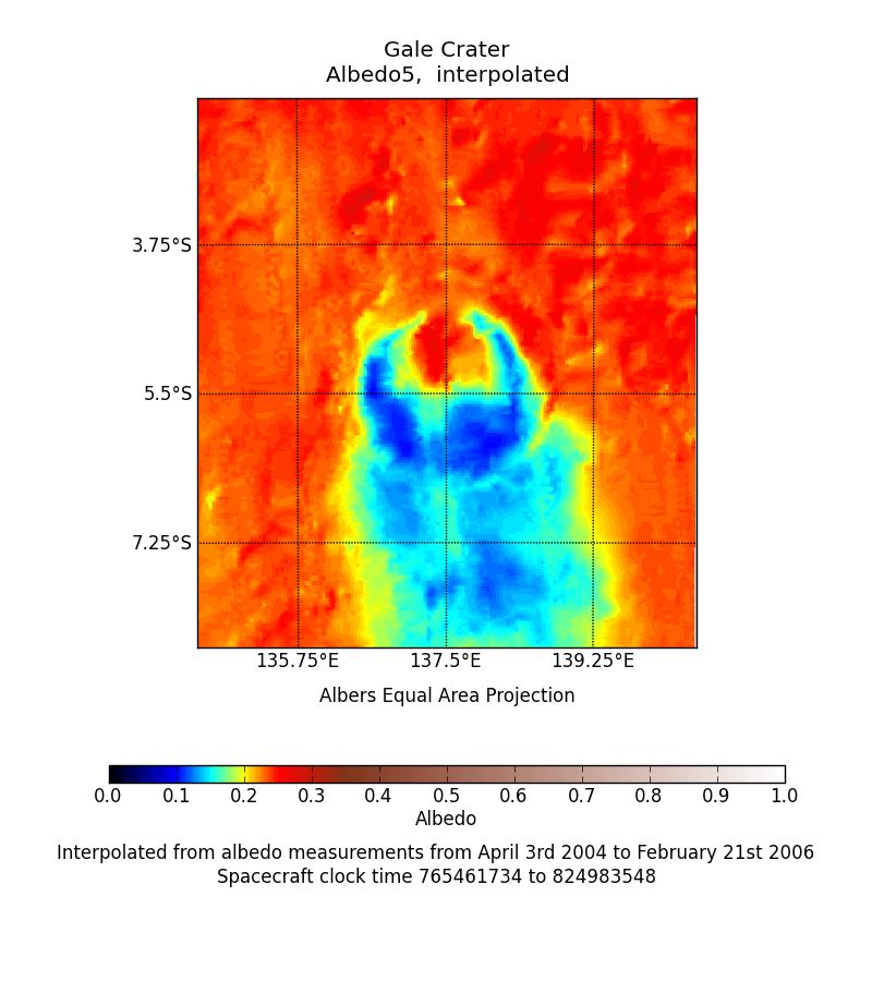
Above images show the 3 maps of albedo measurements for the Gale Crater project, before and after interpolation.
TES Thermal Inertia Maps
Global maps of Thermal Inertia were produced from TES measurements by Putzig and Mellon [2007], using the methods that have developed into those currently employed by this web site. Mean annual maps are available for inertia derived from both Daytime and Nightime measurements. And seasonal inertia from each 10° solar longitude interval is also available for both day and night. Global maps are available on the TES Thermal Inertia page, and these same plots cropped to your project bounds are available from the project bounds.Output Files
Aside from the images, which can be downloaded by right clicking and choosing 'Save Image As...' (or its equivalent for your browser), the data files that store the maps and are used by the THEMIS image processing are available to download as hdf5 files. The data are stored using the python h5py interface: 'Datasets are organised in a filesystem-like hierarchy using containers called 'groups', and accessed using the traditional POSIX /path/to/resource syntax.' The files should be readable by any language capable of reading .hdf files, not just python.The contents of the files depends on the type of file.
| File Type | Example Name | Group | Items | ||||
|---|---|---|---|---|---|---|---|
| Dust Opacity History | Gale_Crater_1_dust.hdf5 | DustOpacityHistory | Item | type | description | ||
| Units | attribute | unitless | |||||
| Minlat | attribute | The minimum latitude used to create the dust opacity. | Maxlat | attribute | The maximum latitude used to create the dust opacity. | ||
| Minlon | attribute | The minimum longitude used to create the dust opacity. | Maxlon | attribute | The maximum longitude used to create the dust opacity. | Dust | data set | The Dust Opacity as a 1D float array. | Ls | data set | The Solar Longitude as a 1D float array.. | SPaceCraftClockTime | data set | The Spacecraft clock time, in seconds since 1st January 1980, as a 1D float array. | Elevation Map | Gale_Crater_1_elev.hdf5 | ElevationMap | Items | type | description |
| Units | attribute | m | |||||
| latitude | data set | The latitude, 1D float array. | longitude | data set | The longitude, 1D float array. | elevation | data set | The elevation at each pixel location, 2D float array. | Albedo Maps | Gale_Crater_1_alb_meas.hdf5 | AlbedoMaps | Items | type | description |
| Units | attribute | None | |||||
| latitude | data set | The latitude, 1D float array. | longitude | data set | The longitude, 1D float array. | albedo1 | data set | The TES measurements of albedo between spacecraft clock time 644004568 and 704113436. The no data value is 0.0. | albedo2 | data set | The TES measurements of albedo between spacecraft clock time 704113437 and 765461734. The no data value is 0.0. | albedo3 | data set | The TES measurements of albedo between spacecraft clock time 765461734 and 824983548. The no data value is 0.0. | TES Thermal Inertia mean Maps | Gale_Crater_1_tes_mean.hdf5 | TesMaps | Items | type | description |
| Units | attribute | tiu | |||||
| latitude | data set | The latitude, 1D float array. | longitude | data set | The longitude, 1D float array. | Daytime_mean | data set | The TES derived thermal inertia. Mean of all day time measurements. The no data value is 0.0. | Nighttime_mean | data set | The TES derived thermal inertia. Mean of all night time measurements. The no data value is 0.0. | TES Thermal Inertia seasonal Maps | Gale_Crater_1_tes_seasonal.hdf5 | TesMaps | Group | type | description |
| Units | attribute | tiu | |||||
| latitude | data set | The latitude, 1D float array. | longitude | data set | The longitude, 1D float array. | Daytime_Ls_=_000-010 | data set | The TES derived thermal inertia. Daytime mean for measurements taken between Ls 0 and 10°. The no data value is 0.0. | Nighttime_Ls_=_000-010 | data set | The TES derived thermal inertia. Nighttime mean for measurements taken between Ls 0 and 10°. The no data value is 0.0. | Daytime_Ls_=_010-020 | data set | The TES derived thermal inertia. Daytime mean for measurements taken between Ls 10 and 20°. The no data value is 0.0. | Nighttime_Ls_=_010-020 | data set | The TES derived thermal inertia. Nighttime mean for measurements taken between Ls 10 and 20°. The no data value is 0.0. | etc etc | data set | For all 10° bands of Ls. |
Reading hdf5 files
Reading hdf5 files with python
To open an hdf5 file in python you can do something like this:
>>> f = h5py.File('file_name', 'r')
Then to access a group:
>>> group = f['group_name']
To access an attribute:
>>> attribute = group.attrs['attribute_name']
To access a data array:
>>> data_array = group['dataset_name']
To see which datasets are available in the group, or file:
>>> for key, value in group.items():
      >>>     print key
Or to see all the attributes:
>>> for key, value in group.attrs.items():
      >>>     print key
So, for example, the following program would work to open and plot the elevation map for the Gale Crater project...
    # Python code to retrieve and plot the elevation map from a
          # project file.
          import h5py
          import numpy as np
          import matplotlib.pylab as plt
          # Open the file
          f_elev = h5py.File('Gale_project/Gale_Crater_1_elev.hdf5','r')
          # Extract the group
          elev_group = f_elev['ElevationMap']
          # Extract the data sets and the attributes.
          units = elev_group.attrs['Units']
          elevation = np.array(elev_group['elevation'])
          latitude = np.array(elev_group['latitude'])
          longitude = np.array(elev_group['longitude'])
          f_elev.close()
          # Plot the output
          plt.figure()
          plt.title('Elevation map of Gale Crater')
          plt.pcolormesh(longitude, latitude, elevation)
          plt.xlim((longitude[0],longitude[-1]))
          plt.ylim((latitude[0],latitude[-1]))
          plt.xlabel('Longitude West')
          plt.ylabel('Latitude North')
          # Create a colorbar
          cb = plt.colorbar(aspect=40)
          # Set the label for the colorbar to be the attribute (units)
          cb.set_label(units)
          plt.show()
Reading hdf5 files with idl
(Use caution, I am not experienced in idl programming, there are probably better ways to achieve the same aims.)
To open an hdf5 file in idl you can do something like this:
IDL> f = H5F_OPEN('file_name')
Then to access a group:
IDL> group = H5G_OPEN(f, 'group_name')
To access an attribute:
IDL> attribute = H5A_OPEN_NAME(group, 'attribute_name')
To access a data array...
IDL> data_array = H5D_OPEN(group, 'dataset_name')
To see which datasets and attributes are available in the file:
IDL> contents = H5_PARSE('file_name')
      IDL> help, contents, /STRUCTURE
Or within a group:
IDL> help, contents.group_name, /STRUCTURE
So, for example, the following program would work to open and plot the derived thermal inertia from a typical themis derived image.
    ; ReadHDF5.pro
          ; idl script that will read the thermal inertia from the requested
          ; file, and plot it in a very basic way.
          pro ReadHDF5
              ; Open the file
              F = H5F_OPEN('filename')
              ; Open the group
              G = H5G_OPEN(F, 'marstherm_data')
              ; Get an attribute
              PixRes = H5A_OPEN_NAME(G, 'PIXELRESOLUTION')
              print, PixRes
              ; Get a dataset
              DataSet_ID = H5D_OPEN(G, 'inertia_array')
              ; and read it
              DataSet = H5D_READ(DataSet_ID)
              ; Plot it
              TV, DataSet
          end
Reading hdf5 files with matlab
To open an hdf5 dataset in matlab you can do something like this:
>> dataset = h5read('file_name', 'data_set_path')
Where 'data_set_path' is the path to the file, e.g. /marstherm_data/inertia_array.
To access an attribute:
>> attribute = h5readatt('file_name', 'data_set_path', 'attribute_name')
To see which datasets and attributes are available in the file:
>> h5disp('file_name')
So, for example, the following program would work to open and plot the derived thermal inertia from a typical themis derived image.
    % matlab script that will read the thermal inertia from the
          % requested file, and plot it in a very basic way.
          %
          % First display the structure of the file.
          h5disp('filename')

          % Get an attribute
          PixRes = h5readatt('filename', '/marstherm_data', 'PixelResolution')
          % Get a dataset
          Inertia = h5read('filename', '/marstherm_data/inertia_array')

          figure()
          imshow(Inertia, [5 5000])
          colorbar()